Papers often use the metrics most familiar to the authors without a systematic assessment of which may be the best for the given purpose. A more holistic assessment of how metrics may assess abundance, range overlap, or even temporal components of how this may change are presented by Gemma using both a case study from Alaska and simulated data. Hopefully this manuscript can serve as a guide for researchers to decide which metric may be best for their purpose when testing predator-prey overlap and how it may change over time.
 G. Carroll, K.K. Holsman, S. Brodie, J.T. Thorson, E.L. Hazen, S.J. Bograd, M.A. Haltuch, S. Kotwicki, J. Samhouri, P. Spencer, E. Willis-Norton, and R.L. Selden, 2019. A review of methods for quantifying spatial predator-prey overlap. Global Ecology and Biogeography, DOI: 10.1111/geb.12984 PDF
Abstract
Background: Studies that attempt to measure shifts in species distributions often consider a single species in isolation. However, understanding changes in spatial overlap between predators and their prey might provide deeper insight into how spe ‐cies redistribution affects food web dynamics.
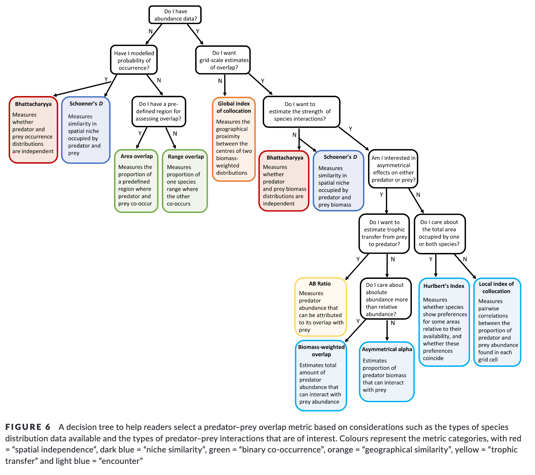
Predator–prey overlap metrics: Here, we review a suite of 10 metrics [range overlap,area overlap, the local index of collocation (Pianka’s O), Hurlbert’s index, biomass‐weighted overlap, asymmetrical alpha, Schoener’s D, Bhattacharyya’s coefficient, the global index of collocation and the AB ratio] that describe how two species overlap in space, using concepts such as binary co‐occurrence, encounter rates, spatial niche similarity, spatial independence, geographical similarity and trophic transfer. We describe the specific ecological insights that can be gained using each overlap metric, in order to determine which is most appropriate for describing spatial predator–prey interactions for different applications.
Simulation and case study: We use simulated predator and prey distributions to demonstrate how the 10 metrics respond to variation in three types of predator–prey interactions: changing spatial overlap between predator and prey, changing predator population size and changing patterns of predator aggregation in response to prey density. We also apply these overlap metrics to a case study of a predatory fish (arrowtooth flounder, Atheresthes stomias) and its prey (juvenile walleye pollock, Gadus chalcogrammus) in the Eastern Bering Sea, AK, USA. We show how the metrics can be applied to understand spatial and temporal variation in the overlap of species distributions in this rapidly changing Arctic ecosystem.
Conclusions: Using both simulated and empirical data, we provide a roadmap for ecologists and other practitioners to select overlap metrics to describe particular aspects of spatial predator–prey interactions. We outline a range of research and management applications for which each metric may be suited.